Do Wolves Control their Own Numbers?
B y L . David Mech
Editor’s note: This story was first published in the winter 2021 issue of International Wolf magazine. Not a member? Join today to receive the next issue of International Wolf plus more great benefits!
When assessing changes in wolf numbers, comparing wolf numbers in various areas or studying what controls wolf numbers, understanding wolf density is key.
In January 2021, gray wolves were removed from the federal Endangered Species List (delisted) except for the Mexican gray wolf. Management of the gray wolf then reverted to individual states. In Montana, Idaho, Wyoming and parts of Washington, Oregon and Utah, wolves were delisted several years earlier, and some of these states soon opened regulated hunting and trapping seasons on the wolves. Managing wolves by opening a season on them, in the same way states manage deer, elk, bears and other wildlife, made many members of the public question why states felt they had to begin controlling wolves.
“Don’t wolves control their own numbers?” these folks asked. Scientists had long pondered that question, and much research has been devoted to the subject. After all, wolf packs are territorial, and the most common natural cause of death is wolves fighting and killing each other while defending those territories. But the question of whether wolves control their own numbers is a trick question, and trying to answer it is not easy.
The trick is that, to start with, one must distinguish between two important concepts regarding wolf numbers: wolf density and wolf population. Wolf density is the number of wolves in an area of a given size—for example, wolves per 1,000 miles2. This measure is not one the public sees very often. Most often, media mention the number of wolves in a state or region, like “2,500 wolves in Minnesota.” That’s a perfectly useful measure for some uses, but not for others.
When assessing changes in wolf numbers, comparing wolf numbers in various areas or studying what controls wolf numbers, understanding wolf density is key. That is because wolf populations can fluctuate in three ways: (1) by increasing or decreasing within a certain area—i.e., a change in density; (2) by occupying a larger or smaller area—i.e., a change in distribution, or (3) by changing in density and distribution.
Most wolf populations that have increased during the last few decades, both in North America and Europe, have done so mainly by spreading to new areas, usually after building up in density. Learning what determines changes in wolf density is key to answering the question of whether wolves control or limit their own numbers.
As long ago as 1967, Canadian biologist Doug Pimlott proposed that wolf numbers were self-limiting. I tended to agree with him in my 1970 book, The Wolf: Ecology and Behavior of an Endangered Species, which is still in print. That conclusion was based on the finding that in many areas where wolves were legally protected, their numbers increased but only to a certain density—about one per 10 square miles, even without humans controlling them.
As years went by, however, more data about wolf populations and their prey accumulated, and the question of whether wolves controlled their own numbers drew more attention. Wisconsin biologist Lloyd Keith decided to test another possibility. Instead of wolves limiting themselves, he wondered if wolves were, like many animals, limited by their food supply. In 1983, he examined the relationship between the number of wolves in an area (wolf density) and the accumulated weight (biomass) of their main prey population in that same area.
By that time, wolf biologists had published studies of seven wolf populations and the numbers of their prey. Keith ran a test of the relationship between the wolf densities in each of those seven studies and the weights of their available prey for each of the same areas. He found a correlation: the greater the amount of prey, the more wolves per area.
A perfect relationship, or correlation of 100%, between those two measures would mean that the amount of prey completely explained the number of wolves. In other words, the number of wolves in a given area was essentially determined, controlled or limited, by the amount of their available food. The correlation Keith found was 64% based on those seven studies. Thus, his findings showed that the available amount of food explained 64% of the differences in the number of wolves per area The remaining amount of difference could be explained by sampling error in the studies, or by an inadequate sample of wolf and prey systems.
After many more published studies of wolf populations and prey numbers produced similar results, one of Keith’s students, Todd Fuller, in 1989 again checked the relationship and found it was even stronger then, based on 25 studies. The new correlation was 72%. In 2003, Fuller teamed up with other authors to examine the relationship based on adding data from seven more studies. Later, other biologists closely examined each of the 32 studies that Fuller and his colleagues included in their latest analysis and realized that some of those 32 wolf and prey populations were subject to human hunting and trapping; other studies involved the eastern wolf, which was considered by some biologists to be a separate species from the gray wolf. Purifying the sample by deleting those studies from the analysis left 26 studies that were still valid to examine for testing the relationship.

In 2015, Shannon Barber-Meyer and I added one more study to the analysis: Yellowstone wolf numbers and the biomass of their main prey, elk. This was an important area to add to the sample of wolf study locations because Yellowstone wolf density was more than 20% higher than any of the others in the sample. If the correlation held up for this higher wolf density, it would render the relationship with available prey even more robust.
Not only did the correlation hold up in Yellowstone; it raised the relationship to 81% (Figure1). Thus, some 81% of the variation in wolf numbers can now be explained by their amount of available food. The strong implication of this finding is that where prey numbers are low, wolf numbers will also be low and vice versa, regardless of the wolves being territorial and killing each other. No doubt these factors, by adjusting wolf numbers, help regulate the wolf population, but they do so in accordance with the prey biomass.
It turns out that, as wolf packs compete for the available prey, their territory sizes simply adjust to the amount of prey and the number of wolves in their packs. The actual number of wolves in the area, however, rises and falls with the amount of their available prey. Wolf numbers simply build up until their population reaches its limit based on the amount of prey; then they spill over into new areas where prey is available. Wolves are highly prolific, with average litter sizes reaching an average of 5.4 pups per breeding pair each year. Because in most areas average pack sizes are about six, these populations basically double each spring. The surplus wolves, i.e., the number that exceed the food supply, are the maturing pups. As they grow older, they disperse away from their packs to other areas where there is prey but no wolves yet. Both sexes disperse, often for hundreds of miles.
When these dispersers find a member of the opposite sex that has also emigrated, they can bond with each other and form a breeding pair (formerly called an “alpha pair”). Because most of the areas surrounding wolf populations host plenty of deer and other prey, most places where dispersing wolves end up support sufficient food. There the pair can set up a new territory and produce pups, thus starting their own pack.
An excellent example of this process is currently playing out in the western United States. Wolf numbers in Idaho, Montana and Wyoming have been increasing for years and spilling over into Washington and Oregon, with some of Oregon’s wolves dispersing into California. In 2021, the northern Rocky Mountain population also started to recolonize Colorado.
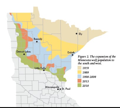
The same thing happened in the Midwest decades ago when Minnesota’s wolf population built up. That population had never been exterminated from the northeastern corner of the state, a large wilderness contiguous to Ontario’s wilderness. After Minnesota ended its wolf bounty and later, after wolves were legally protected by the federal Endangered Species Act, the increasing population flowed over into Wisconsin to its east and then into Michigan. It also spread father south and west within Minnesota (Figure 2).
However, that process in the Midwest took place more slowly. Minnesota’s wolves were classified as threatened rather than endangered since 1978, and that classification allowed the federal government’s Wildlife Services to remove wolves preying on livestock there. Most such depredations occur along the frontier of the wolf’s range. Thus, the number of wolves that are trying to repopulate that frontier is artificially constrained if they are killed for taking livestock. Nevertheless, wolf distribution has still been expanding within Minnesota—just more gradually now.
These examples are typical of the behavior of wolf populations and demonstrate that wolves do not control their own populations. But what about wolf density? Don’t wolves control their own density as dictated by prey abundance? Yes—in many ways. However, they primarily do so by spilling over into new areas through dispersal of young wolves, thus increasing their population. With numbers determined by their food supply, and prey widely distributed and abundant, wolf populations easily proliferate. Deer, elk, moose, wild boar, caribou or other wolf prey are common in many regions. Thus, wolf populations naturally repopulate as much area as their food supply allows, and they can be expected to do so until they conflict too much with human interests. In those places and at those times, the tendency has been for humans to try to assert control.
Primary References Used
Fuller, T.K. 1989. Population dynamics of wolves in north-central Minnesota. Wildl. Monogr. No. 105.
Fuller, T.K., Mech, L.D., and Fitts-Cochran, J. 2003. Wolf population dynamics. In Wolves: behavior, ecology, and conservation. Edited by L.D. Mech and Boitani. University of Chicago Press, Chicago, Ill. pp. 161–191.
Keith, L.B. 1983. Population dynamics of wolves. In Wolves in Canada and Alaska: their status, biology, and management. Edited by L.N. Carbyn. Can. Wildl. Serv. Rep. Ser. No. 45. Canadian Wildlife, Edmonton, Alta. pp. 66-77.
Mech, L. D. and S. M. Barber-Meyer. 2015. Yellowstone Wolf (Canis lupus) Density Predicted by Elk (Cervus elaphus) Biomass. Can. J. Zoology. 93(6): 499-502, 10.1139/cjz-2015-0002